| code0 | code | format | type | Lat | Lon | StartTime | EndTime |
|---|---|---|---|---|---|---|---|
| missing | ZB | 知本 | GM | 22.7398 | 121.065 | 20201006 | missing |
| missing | XC | 新城 | GM | 24.0383 | 121.609 | 20201006 | missing |
| missing | SM | 日月潭 | GM | 23.881 | 120.908 | 20191008 | missing |
| missing | CN | 暨南 | GM | 23.9576 | 120.928 | 20221229 | missing |
| em3 | KUOL | 過嶺 | GE | 24.9629 | 121.142 | 2011-09-22 | 9999-12-31 |
| em4 | HUAL | 華陵 | GE | 24.6745 | 121.368 | 2012-01-17 | 9999-12-31 |
| em5 | TOCH | 頭城 | GE | 24.8435 | 121.805 | 2012-02-10 | 9999-12-31 |
| em6 | ENAN | 南澳 | GE | 24.4758 | 121.785 | 2012-02-15 | 9999-12-31 |
| ⋮ | ⋮ | ⋮ | ⋮ | ⋮ | ⋮ | ⋮ | ⋮ |
Tutorial
Requirements
環境
GEMS-MagTIP 依賴以下工具箱; 在 MATLAB 指令列中輸入 license('inuse') 或 ver 可以列出您電腦上目前可用的工具箱。
Toolbox in-use:
- MATLAB Version 9.11 (R2021b)
- Mapping Toolbox Version 5.2 (R2021b)
- Parallel Computing Toolbox Version 7.5 (R2021b)
- Signal Processing Toolbox Version 8.7 (R2021b)
- Statistics and Machine Learning Toolbox Version 12.2 (R2021b)
Dependencies
GEMS-MagTIP 依賴於 okatsn/toolbox 和 CGRG-lab/GEMS-MagTIP-insider。
在執行腳本前,您需要將這些依賴項加入系統的路徑設定,如下所示:
CGRG-lab/GEMS-MagTIP-insider
將 CGRG-lab/GEMS-MagTIP-insider 複製到本地磁碟中 (例如 GEMS-MagTIP-insider),並將其內的原始碼加入系統路徑:
dir_src = 'GEMS-MagTIP-insider/src';
addpath(genpath(dir_src));
okatsn/toolbox
將 okatsn/toolbox 複製到主目錄中 (例如 GEMS-MagTIP-insider/toolbox),並將其內的原始碼加入系統路徑:
dir_toolbox = 'GEMS-MagTIP-insider/toolbox';
addpath(genpath(dir_toolbox));
Getting Started
GEMS-MagTIP 的主要函數 需要以目錄中的中間數據(如 .mat 文件)作為輸入參數,並將輸出數據存放於指定的目錄中。
以下是一個主要函數操作鏈的簡單示例:
準備數據
您需要準備/更新以下數據:
- 地震目錄
- 標準格式的地電數據
- 標準格式的地磁數據
地震目錄與測站資訊
請下載或更新 GDMSN 的地震事件目錄,其中規模 (M_L ),並將其儲存至 spreadsheet/catalog.csv。 檔案 spreadsheet/station_location.csv 用於指定每個測站的位置,它直接包含在GEMS-MagTIP-insider的目錄下。
要點:
- 標題名稱:
catalog.csv:標題必須是 ‘time’、‘Lon’、‘Lat’、‘Depth’ 和 ‘Mag’。station_location.csv:標題必須是 ‘code’、‘format’、‘Lon’ 和 ‘Lat’。- 欄位名稱的排列順序可以隨意,但名稱字串必須完全一致。
- 更新地震目錄:
- 要更新地震目錄,將更新的表格以 CSV 格式儲存至
spreadsheet/catalog.csv,並啟用覆寫。 - 執行
checkcatalog(dir_catalog)來處理新的目錄。 - 如果
dir_catalog資料夾中同時存在catalog.mat和catalog.csv,則將使用更新的catalog.csv資料覆寫生成catalog.mat。
- 要更新地震目錄,將更新的表格以 CSV 格式儲存至
- 更新測站位置:
- 將更新的測站位置表格儲存至
spreadsheet/station_location.csv,並啟用覆寫。 - 遵循與更新地震目錄相同的工作流程。
- 將更新的測站位置表格儲存至
支援的目錄格式
GDMSN 格式
| date | time | lat | lon | depth | ML | nstn | dmin | gap | trms | ERH | ERZ | fixed | nph | quality |
|---|---|---|---|---|---|---|---|---|---|---|---|---|---|---|
| … | … | … | … | … | … | … | … | … | … | … | … | … | … | … |
自由格式
| time | Lon | Lat | Depth | Mag |
|---|---|---|---|---|
| 2020/8/10 06:41 | 121.59 | 23.81 | 29.86 | 3.41 |
| 2020/8/10 06:29 | 120.57 | 22.18 | 43.54 | 3.02 |
| 2020/8/10 06:14 | 121.7 | 22.17 | 124.78 | 4.13 |
| … | … | … | … | … |
以下為 station_location.csv 的部分內容範例:
標準格式資料
將原始數據轉換為標準格式非常重要。 此轉換過程包括日期時間驗證、將地電數據投影為NS-EW格式、格式化文件名稱以供索引等。
以下是一個將原始數據轉換為標準格式的簡單腳本:
dir_gems_raw = 'data-raw/GEMSdat'; % raw GEMS data
dir_mag_raw = 'data-raw/MAG'; % raw MAG data
dir_data = 'data-standard'; % output directory
conv_gemsdata(dir_gems_raw, dir_data, dir_catalog);
conv_geomagdata(dir_mag_raw, dir_data);
Tip
您可以自由整理放置標準格式資料的 dir_data 中的文件和文件夾,也不必擔心對同一原始數據進行多次轉換會發生錯誤,因為在 GEMS-MagTIP 中數據讀取依賴於標準格式的文件名,而檔案轉換函數會自動處理重複的文件。
參閱 standarddataname 和 write_data。
有關更多資訊,請參閱讀取原始數據並將其轉換為標準格式部分。
設置目錄路徑
在運行任何主要函數之前,必須分配輸入/輸出數據或變量的目錄。
例如:
% For windows, use backslash `\`; for unix systems, use slash `/` in the path to directories.
dir_catalog = 'GEMS-MagTIP-insider/spreadsheet';
        % directory of event catalog & station location
dir_data = 'standard-data';
        % directory of geomagnetic timeseries of "standard format"
dir_stat = 'var-output/StatisticIndex';
        % directory of statistic indices
dir_tsAIN = 'var-output/tsAIN';
        % directory for storing anomaly index number (AIN)
dir_molchan = 'var-output/Molchan';
        % directory for storing Molchan scores
dir_jointstation = 'var-output/JointStation';
        % directory for the time series of EQK, TIP and probability
Tip
- 您可以使用
mkdir_default自動生成主要函數所需的空目錄。 - 您可以使用
dirselectassign通過文件瀏覽器界面分配目錄。
Important
dir_catalog必須包含catalog.csv或catalog.mat,以及station_location.csv或station_location.mat。dir_data是包含 GE 或 GM 標準格式資料的目錄;請參閱conv_geomagdata和conv_gemsdata以將原始數據轉換為標準格式。
按正確的順序執行主要函數
statind(dir_data,dir_stat);

anomalyind(dir_stat,dir_tsAIN);

molscore(dir_tsAIN,dir_catalog,dir_molchan);

molscore3(dir_tsAIN,dir_molchan,dir_catalog,dir_jointstation);
Tip
statind、molscore 和 molscore3 有平行計算的替代方案。 在大多數情況下,您只需在函數名稱後附加 _parfor (例如,molscore3_parfor(...)) 即可在不修改輸入參數的情況下進行平行運行。 參閱 statind_parfor、molscore_parfor 和 molscore3_parfor。
綜合範例腳本
以下是整個流程的範例腳本 “demo/demo_script.m”。
Tip
您可以運行 startup0.m 並按照命令視窗中的指示,添加依賴項並分配如上所述的輸入/輸出目錄。
%% Convert Raw data to standard type
% Load original data and save them as matfiles of the standard format

conv_gemsdata(dir_gems_raw, dir_data, dir_catalog,'FilterByDatetime',datetime(2020,1,1)); % Convert raw GE data of timestamps after 2020-1-1 to standard format.
% Assign 'FilterByDatetime' to save time when standard geomagnetic data out of the specified date-time range already exist.
% Discard 'FilterByDatetime' to convert everything in the raw-data directory.
conv_geomagdata(dir_mag_raw, dir_data,'FilterByDatetime',datetime(2020,1,1)); % The same as above but for the conversion of GM data.

%% Calculate Statistic Index
statind_parfor(dir_data,dir_stat, ... % Load data in dir_data, save index in dir_stat
    'Preprocess',{'ULF_A','ULF_B','BP_40','BP_35'}, ... % with 4 kinds of filtering
    'SavePreprocessedData',false, ... % without saving filtered timeseries
    'StatName', {'S', 'K', 'FI', 'SE'},  ... % the variable name for 'StatFunction'.
    'StatFunction', {@skewness, @kurtosis, @fisherinformation, @shannonentropy}, ...
    'FilterByDatetime',[datetime(2011,1,1), datetime(2022,12,31)]);
% Assign 'FilterByDatetime' to calculate statistical indices only between 2011-1-1 and 2022-12-31.
% Noted that standard format GE/GM data have to be available in this range, otherwise you will get NaN if data is missing (or not converted) in `dir_data`.


%% Data overview
% An overview of data avaliability/deficiency according to the results in dir_stat
plot_dataoverview(dir_stat, dir_catalog);

%% Calculate Anomaly Indices
anomalyind(dir_stat,dir_tsAIN);

%% Training
molscore_parfor(dir_tsAIN,dir_catalog,dir_molchan,...
    'TrainingPhase', {calyears(3),datetime(2022,4,1);... % Use up to 3-years data before 2022-4-1 for model training.
                      calyears(5),datetime(2022,4,1);... % Use up to 5-years data before 2022-4-1 for model training.
                      calyears(7),datetime(2022,4,1);... % Use up to 7-years data before 2022-4-1 for model training.
                      calyears(9),datetime(2022,4,1)},...% Use up to 9-years data before 2022-4-1 for model training.
    'modparam',{'Test', 5000}); % Remember to disable 'Test' in a real run.

%% Forecast and test
molscore3_parfor(dir_tsAIN,dir_molchan,dir_catalog,dir_jointstation,...
    'OverwriteFile',true, ...
    'ForecastingPhase', repmat([datetime(2022,4,2), datetime(2022,9,27)], 4,1));
    % Manually assign forecasting phases. Typically the size of 'ForecastingPhase' should align with the size of 'TrainingPhase'.
結果可視化
See also: Plotting functions
繪製EQK-TIP 匹配圖
繪製每個測站的 EQK-TIP 匹配圖:
%% Plot EQK-TIP of each station

% the output directory for the images
dir_png = fullfile(dir_molchan,'png','EQKTIP'); % no need to mkdir

% Plot TIP of individual stations as heatmap,
% with target earthquakes (EQK) scattered on the top.
plotEQKTIP1(dir_tsAIN,dir_molchan,dir_catalog,dir_png); %,...
    'ForecastingPhase',calyears(1),'ShowTrainingPhase',1,'Rank',1,...
    'ForceMagnitude',false, ...
    'scatter',1);

% remove the white space around the image.
cropimg(dir_png,'SaveInplace',true);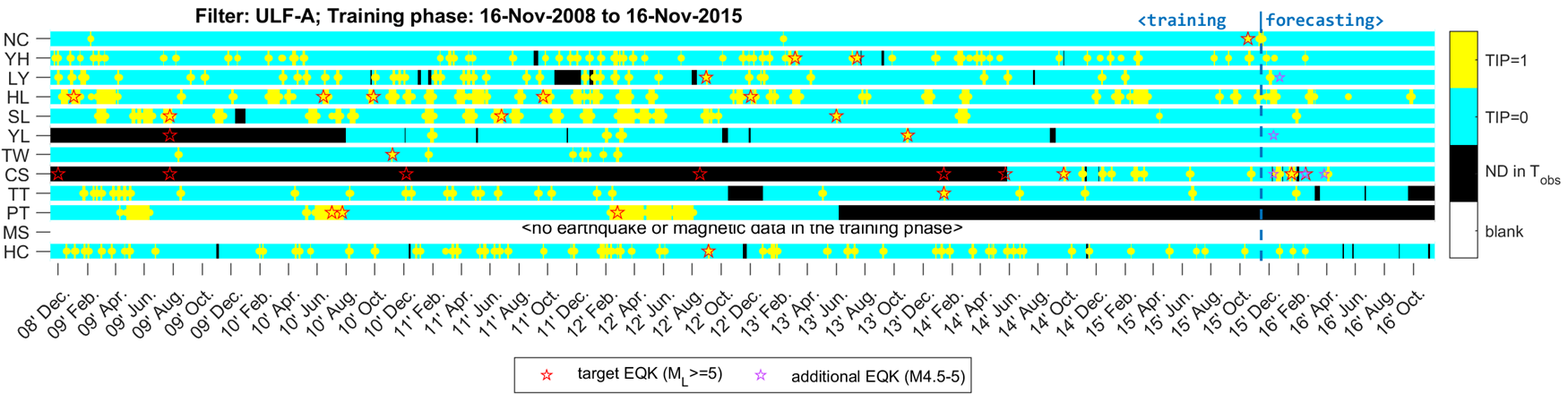
在此圖中,展示了由各測站最佳模型(rank 1)定義的EQK與TIP的匹配圖。黑色間隔表示在這些日期中 \(T_\text{obs}\) 完全沒有資料(即此模型在這些時間點無資料可供計算),因此無法計算TIP。
繪製二維 EQK-TIP 匹配圖
EQK-TIP 在 2D 時間-空間座標系統中的表示
%% EQK-TIP in a 2D temporal-spatial coordinate system

dir_png = fullfile(dir_jointstation,'png', 'EQKTIP3'); mkdir(dir_png);

% Find the data of ID 'AMn6ei' and filter tag 'ULF_A'

jid = 'AMn6ei';
filter_tag = 'ULF_A';

jpathlist = datalist(sprintf('[JointStation]ID[%s]prp[%s]*.mat', jid, filter_tag), dir_jointstation).fullpath;

% Retrieve essential data from '[JointStation]' files in the jpathlist:

[AlarmedRate, MissingRate,xlabels, EQKs, TIP3s, TIPv3s, TIPTimes, LatLons] = ...
    calcFittingDegree(jpathlist);

% Plot EQK-TIP on a 2D temporal-spatial coordinates

titletag = sprintf('EQK-TIP (trial ID: %s; filter: %s)', jid, filter_tag)
plotEQKTIP3(dir_png, titletag, xlabels, EQKs, TIP3s, TIPv3s,TIPTimes, LatLons);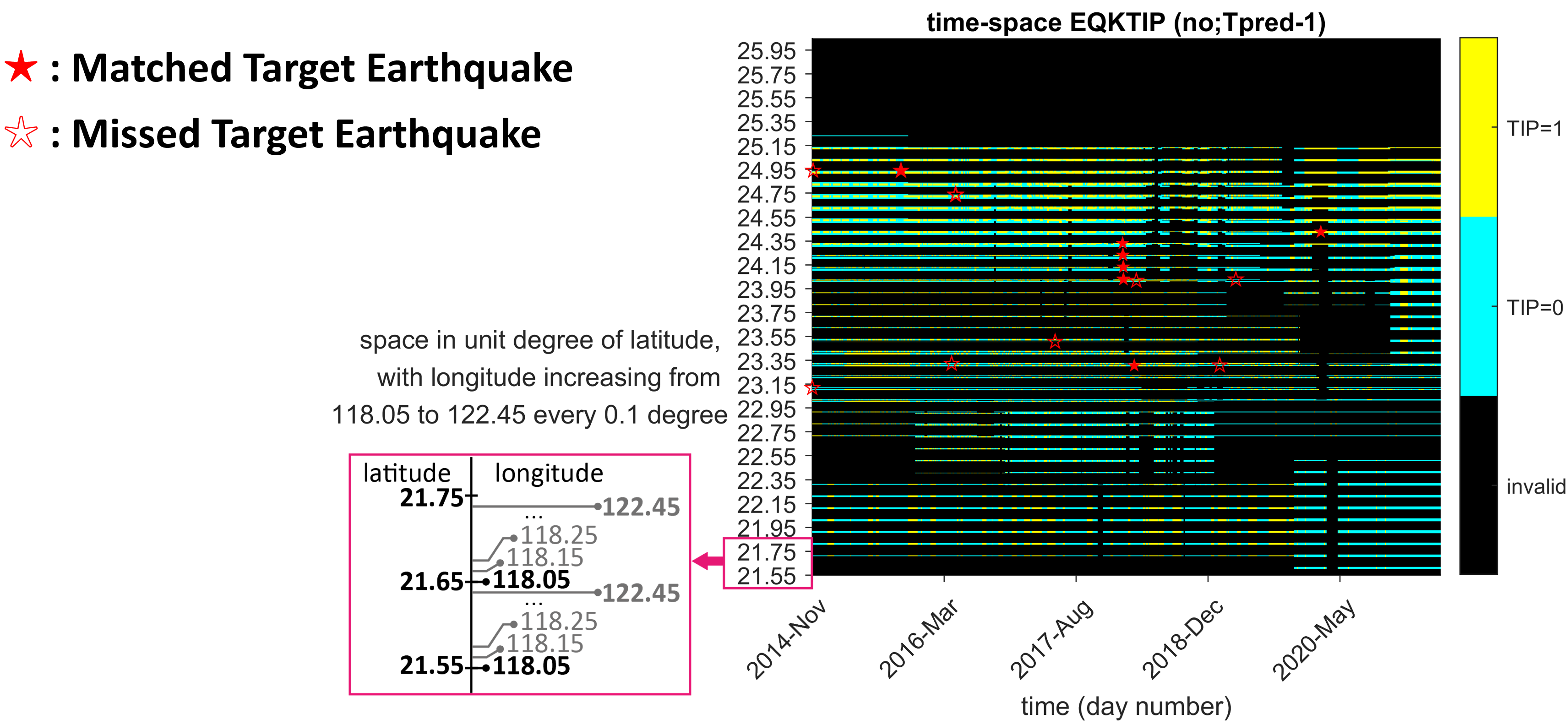
繪製擬合程度
%% Plot fitting degree

dir_png = fullfile(dir_jointstation,'fitting_degree'); mkdir(dir_png);

plotFittingDegree(dir_jointstation,dir_catalog,dir_png,...
    'ConfidenceLevel',0.95);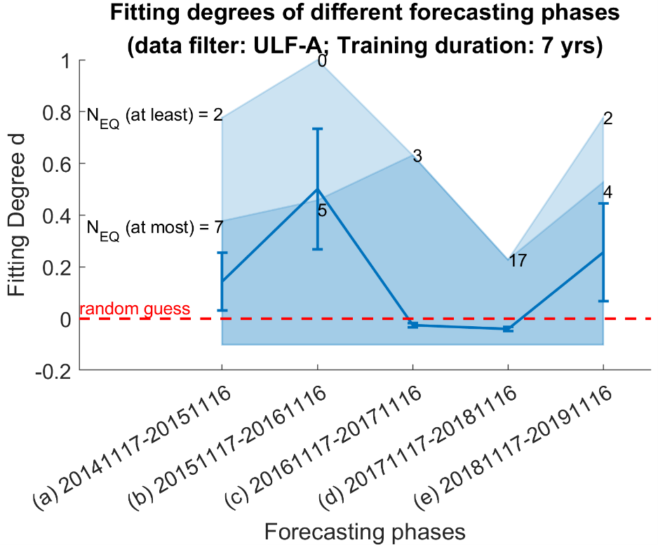
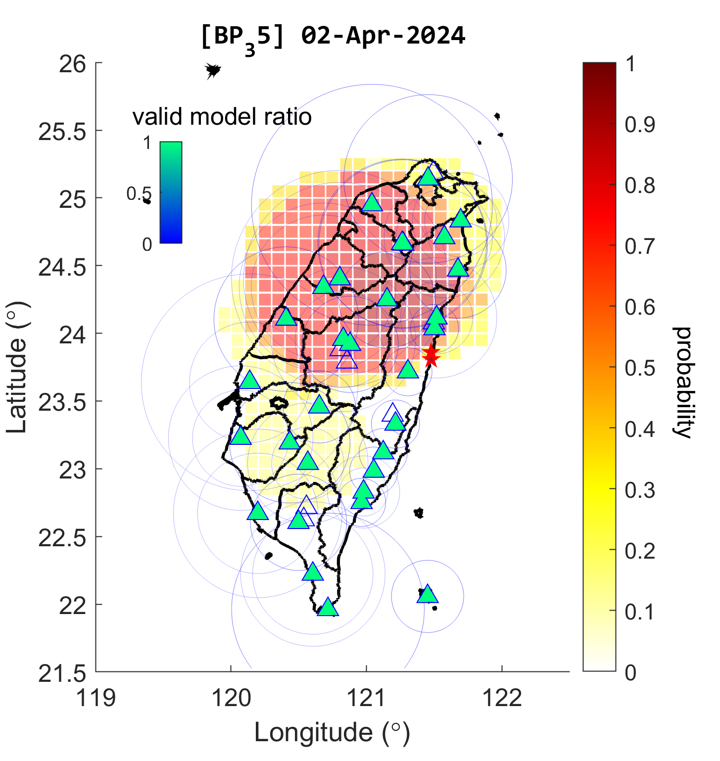
繪製機率圖
%% Plot probability map

% the output directory for the images
dir_prob = fullfile(dir_jointstation,'png','prob');

% specific datetime to be plotted
dates2plot = [datetime(2020,12,1):caldays(30):datetime(2021,2,11)]';

% plot GEMS-MagTIP probability map
% (export individual image for each date)
dir_prob2 = plotProbability(dir_jointstation,dir_catalog,dir_prob, ...
            'TimeRange',dates2plot,...
            'PlotEpicenter','all');
);